How the memory is advanced

The representation chooses the memory modes. The formulation chooses how they are advanced alongside the physical solve. FullHistory is an alternative to both: it keeps the history itself.

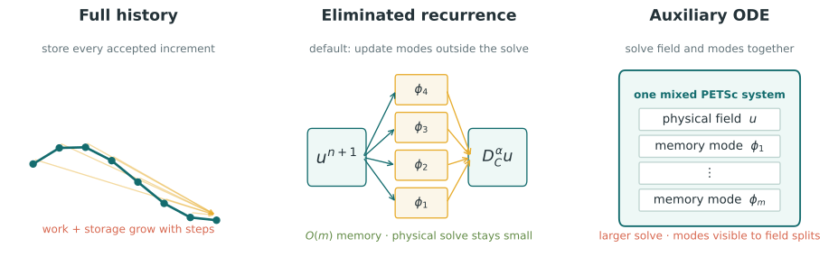
The same fractional derivative can store its full past, eliminate a fixed set of memory modes outside the field solve, or expose those modes in one mixed system.

Eliminated recurrence (default)

Recurrence() advances each mode outside the Firedrake solve. Its default quadratic interpolant uses a quadratic through the current step and the preceding accepted value. For equal steps, the exact variation-of-constants update is

\[ \phi_j^{n+1} =e^{-\lambda_jh}\phi_j^n +A(\lambda_jh)(u^{n+1}-u^n) +Q(\lambda_jh)(u^n-u^{n-1}), \]

where

\[ A(z)=\tfrac12\phi_1(z)+\psi(z),\qquad Q(z)=\tfrac12\phi_1(z)-\psi(z),\qquad \psi(z)=\frac{1-\phi_1(z)}{z}. \]

The first step uses the linear update because no preceding increment exists, which does not change the asymptotic orders. Unequal accepted steps use the corresponding variable-step quadratic coefficients.

Set Recurrence(interpolant="linear") to use the original piecewise-linear assumption,

\[ \phi_j^{n+1} =e^{-\lambda_jh}\phi_j^n +\phi_1(\lambda_jh)(u^{n+1}-u^n). \]

On smooth solutions the observed orders through the stepper are \(2-\alpha\) for linear and \(3-\alpha\) for quadratic. On the singular solutions time-fractional problems usually produce, both are approximately first order and the error is dominated by the first step. Grading the time levels typically helps a singular solution far more than the interpolant does.

The Caputo-Wismer application keeps a dedicated linear modal update.

Auxiliary ODE

AuxiliaryODE puts every mode into one mixed problem on \(V^{m+1}\),

\[ \dot\phi_j+\lambda_j\phi_j=\dot u,\qquad D^\alpha_Cu\approx\sum_jw_j\phi_j , \]

discretized with backward Euler or trapezoidal stepping. This makes the memory variables visible to PETSc. Field-split metadata is exposed through stepper.appctx["yonderdrake"]. See Solvers, field splits, and MPI. This formulation enlarges every solve. The eliminated recurrence is usually cheaper. Both use \(O(m)\) storage.

Backward Euler is first order and trapezoidal approximately second order on smooth solutions. Both fall to first order on a \(t^\alpha\) initial singularity, where trapezoidal offers no general advantage. Every choice here is substantially more expensive per step than the eliminated recurrence, so reach for AuxiliaryODE when PETSc needs access to the memory fields rather than for accuracy.

Sine diffusive oscillator

Oscillator() is the dedicated formulation for SineDiffusive. Every mode has a position and velocity. Under the same piecewise-linear solution assumption, Yonderdrake applies the exact rotation

\[\begin{split} \begin{bmatrix}\omega^{n+1}\\\dot\omega^{n+1}\end{bmatrix} = \begin{bmatrix} \cos(zh)&\sin(zh)/z\\ -z\sin(zh)&\cos(zh) \end{bmatrix} \begin{bmatrix}\omega^n\\\dot\omega^n\end{bmatrix} +\text{linear Duhamel forcing}. \end{split}\]

This formulation uses two fields per mode and supports variable steps. The rotation is undamped, so old mode error persists. It is available only with the comparison-only sine diffusive representation.

Full history

FullHistory() integrates the piecewise-linear solution history against the Caputo kernel directly. This is the variable-step L1 method:

\[ D_C^\alpha u(t_n)\approx \frac1{\Gamma(2-\alpha)} \sum_{k=0}^{n-1} \frac{u_{k+1}-u_k}{t_{k+1}-t_k} \left[ (t_n-t_k)^{1-\alpha}-(t_n-t_{k+1})^{1-\alpha} \right]. \]

There is no quadrature spectrum to tune, which makes it the natural reference when you want a single error source. The cost is that work and storage grow with the number of accepted steps: one stored increment per step. See Lin and Xu (2007) for the classical L1 construction. Yonderdrake evaluates the same history integral on variable steps.

Riemann-Liouville markers add their exact initial-trace term to whichever of these paths is in use.