Caputo-Wismer imaging
The application layer advances the conservative heterogeneous model
Each material supplies an indicator \(\chi_m\), density \(\rho_m\), wave speed \(c_m\), damping coefficient \(b_m\), and fractional order \(\alpha_m\). The indicators normally partition the domain.
from yonderdrake.applications import (
    CaputoWismerImpedanceBoundary,
    CaputoWismerMaterial,
    CaputoWismerModel,
    SensorArray,
)

materials = (
    CaputoWismerMaterial(
        indicator=tissue_mask,
        density=tissue_density,
        wave_speed=tissue_wave_speed,
        damping=tissue_damping,
        alpha=tissue_alpha,
    ),
)
sensors = SensorArray.ring(
    V,
    num_sensors=64,
    radius=0.9,
    width=0.04,
)
outer_boundary = CaputoWismerImpedanceBoundary(
    coefficient=1.0 / (bath_density * bath_wave_speed),
)
model = CaputoWismerModel(
    V,
    materials=materials,
    sensors=sensors,
    boundaries=(outer_boundary,),
    dt=dt,
    num_steps=num_steps,
    num_modes=32,
)
result = model.propagate(initial_pressure)
data = result.sensor_data
result.final_pressure is the final field. Pass record_history=True to
retain every pressure field in result.field_history. Models without PML use
the centred wave update by default, so dt must satisfy the usual finite
element wave CFL restriction. Set stiffness_theta between zero and one to
move the spatial stiffness into the implicit solve.
Sensors
The user controls the sensor count, placement, and averaging width.
ring = SensorArray.ring(V2, 64, radius=0.9, width=0.04)
sphere = SensorArray.sphere(V3, 128, radius=0.9, width=0.06)
custom = SensorArray(V2, locations_xy, width=0.04)
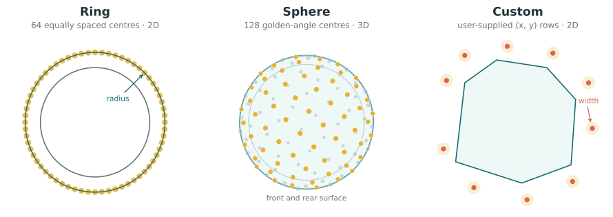
The constructors place sensor centres. width controls the local averaging
footprint around each centre. The small 3D panel is an orthographic view of the
spherical arrangement.
The sphere uses an approximately uniform golden-angle arrangement. Custom
locations contain one (x, y) or (x, y, z) row per sensor.
sensors.locations contains the positions used by the model. The pressure and
sensors share one scalar continuous Lagrange space. CG1 and CG2 are both
supported in 2D and 3D.
Acoustic sources
A source has a spatial profile and one signal value at every model time, including time zero.
from yonderdrake.applications import (
    CaputoWismerArraySource,
    CaputoWismerSource,
)

pulse = CaputoWismerSource.volume(source_profile, signal)
incoming_flux = CaputoWismerSource.boundary(
    boundary_profile,
    boundary_signal,
    boundary_id=3,
)
array_drive = CaputoWismerArraySource(
    array=sensors,
    signals=independent_sensor_signals,
)

driven_model = CaputoWismerModel(
    V,
    materials=materials,
    sources=(pulse, incoming_flux, array_drive),
    dt=dt,
    num_steps=num_steps,
)
Volume and boundary sources enter the weak load directly. An array source uses the exact transpose of sensor sampling. This is useful for controlled emission and sensor-trace backpropagation.
Open boundaries
With neither boundaries nor pml, the weak form has a reflecting natural
boundary. CaputoWismerImpedanceBoundary adds the first-order condition
where \(\eta=1/(\rho c)\) is the outgoing plane-wave value for a homogeneous
exterior medium. Set boundary_id when only one marked part of the boundary
uses the condition. A CaputoWismerSource.boundary(...) supplies \(g\).
For an open-domain calculation, extend the mesh beyond the physical region and place a perfectly matched layer in the extension.
from yonderdrake.applications import CaputoWismerPML

pml = CaputoWismerPML.box(
    mesh,
    interior_bounds=((-1.0, 1.0), (-1.0, 1.0)),
    reference_speed=bath_wave_speed,
    reflection=1.0e-6,
    polynomial_order=3,
)
model = CaputoWismerModel(
    V,
    materials=materials,
    sensors=sensors,
    pml=pml,
    dt=dt,
    num_steps=num_steps,
)
The outer mesh bounds define the end of the layer. The interior bounds define
where directional damping begins. Use a homogeneous bath material throughout
the layer and choose its speed as reference_speed. The real-valued auxiliary
differential equation formulation works in 2D and 3D. PML models use an
implicit first-order pressure and velocity update. They add one directional
field per spatial axis and, in 3D, one pressure-integral field. These fields
participate in the exact discrete adjoint.
PML reduces outgoing reflections but costs more than the scalar pressure update. A first-order impedance boundary is useful when the mesh cannot be extended or the extra PML fields are not justified.
Reconstruction
The same model object defines the forward map and its transpose, so materials, PML fields, boundary conditions, time stepping, and sensor normalization cannot drift between the two.
from yonderdrake.applications import (
    CaputoWismerInverseProblem,
    reconstruct_initial_pressure,
)

problem = CaputoWismerInverseProblem(
    model,
    data,
    regularization=1.0e-6,
)
result = problem.solve(
    max_iterations=100,
    tolerance=1.0e-5,
    positivity=True,
)
image = result.pressure

quick_backprojection = reconstruct_initial_pressure(
    model,
    data,
    method="adjoint",
)
The iterative method uses a scaled adjoint warm start, positivity by default,
and a 100-iteration safety cap. It stops earlier when the optimizer reaches
the default tolerance of 1e-5. Both defaults are user-overridable. The
result records convergence, objective history, function evaluations, and
forward and adjoint timings.
method="adjoint" applies a single exact discrete transpose. It is useful as
a quick image and as a diagnostic, but it does not minimize the sensor misfit.
Time reversal and attenuation compensation
Sensor traces can also be backpropagated through a modified acoustic model.
from yonderdrake.applications import time_reverse_sensor_data

lossless_time_reversal = time_reverse_sensor_data(
    model,
    data,
    compensate_attenuation=False,
)
compensated_time_reversal = time_reverse_sensor_data(
    model,
    data,
    compensate_attenuation=True,
    filter_order=2,
)
Lossless time reversal removes the attenuation term during backpropagation.
Attenuation compensation reverses its sign. That inverse evolution amplifies
high spatial frequencies, so Yonderdrake applies a self-adjoint Helmholtz
filter to the complete implicit and explicit attenuation action at every
step. The filter is part of the coupled solve and its exact transpose. A
direct model with attenuation="reversed" therefore requires
attenuation_filter_length. If filter_length is omitted from
time_reverse_sensor_data, it defaults to 1.5 times the largest cell diameter.
Refine the mesh and vary the filter length when assessing image resolution and
stability.
Gallery
The sensor-array vessel imaging gallery applies these tools to layered and anatomical head models. The forward attenuation model follows Wismer (2006). The iterative inverse method follows Kaltenbacher and Schlintl (2022). The PML uses the real-valued formulation of Kaltenbacher, Kaltenbacher, and Sim (2013).