Gallery

Larger applications producing animations or figures and replot-ready CSV data. Every entry says what to watch for as the solution evolves and decays.

Every entry is an ordinary Python script with a main() function. The scripts live in the repository rather than the installed package, so clone it to run them, then use the Python interpreter from an active Firedrake environment containing the plotting extra:

git clone https://github.com/TSGut/yonderdrake.git
cd yonderdrake
python -m pip install '.[visual]'
python demos/gallery/<script>.py

Outputs land in demos/demo-output/. Data setup and parallel execution for the head demos are described in Head-model data and parallel runs. Use Refinement workflow before treating a result quantitatively.

Fractional time

Fractionally damped waves on a dragon

visual_time_derivative_dragon_wave.py models Caputo-Wismer-Kelvin damping on a dragon mesh. Watch the wave front: classical Kelvin-Voigt damping attenuates high frequencies immediately, while the fractional term keeps a long tail of memory, so the surface keeps ringing after the front has passed. The governing equation, material model, forward solver, and inverse applications are developed in the Caputo-Wismer imaging application.

The fractional model keeps a visible wake after the leading wave front has crossed the dragon.

Three time derivatives, one problem

visual_time_derivative_phase_separation.py solves Allen-Cahn on a sphere with three different time derivatives side by side.

Identical initial data evolve at different coarsening rates under the three time derivatives.

A moving heat source on a torus

In visual_time_derivative_thermal_scanner.py, a source sweeps the surface and the trailing thermal wake shows how far back the memory reaches.

The wake behind the moving source makes the different memory laws directly visible.

Anatomical head models

visual_brainweb_wismer_sources.py places three sources in a BrainWeb anatomical head with material-dependent Caputo-Wismer damping. The companion visual_brainweb_wismer_pulse.py sends a single pulse through the same anatomy, and the two skullball variants use a stylized layered domain with an absorbing outer boundary. Each compares layered, homogenized, and difference fields.

These four run distributed. See Head-model data and parallel runs.

BrainWeb pulse: layered and homogenized tissue models with their absolute difference.

BrainWeb sources: material-dependent damping changes the field relative to the homogenized model.

Skull-ball pulse: the self-contained layered geometry isolates the material-model comparison.

Skull-ball sources: the difference panel shows where heterogeneity most changes the wave field.

Sensor-array vessel imaging

These inverse problems reconstruct a vessel excitation inside a heterogeneous head from pressure recorded by an exterior sensor array. The forward model, sensor geometries, reconstruction methods, and complete examples are covered in Caputo-Wismer imaging.

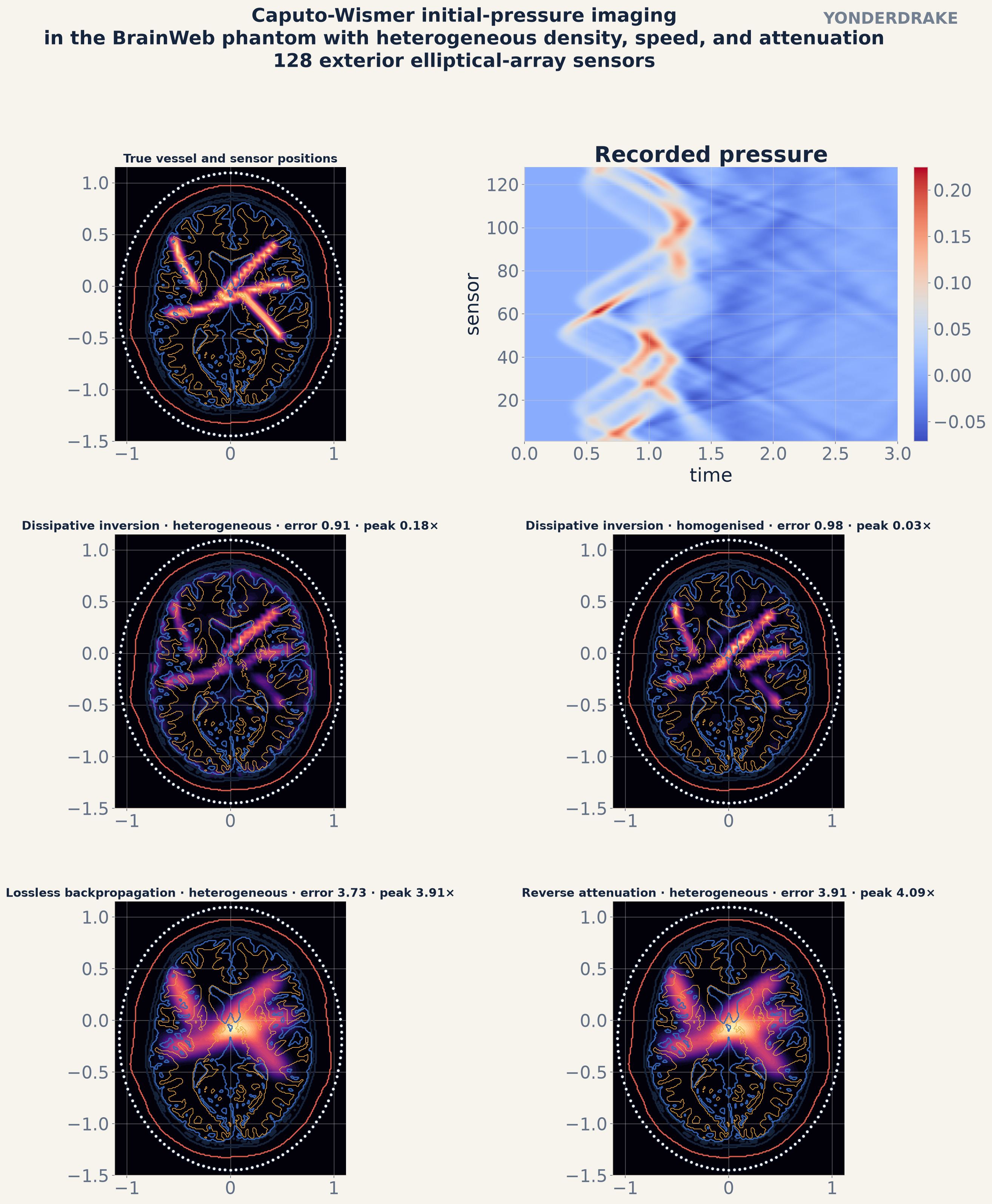
A vessel-shaped initial pressure propagates through the BrainWeb anatomy to an exterior elliptical sensor array. The middle row compares attenuation-aware inversion with the correct heterogeneous anatomy and a homogenized material assumption. The lower row uses the heterogeneous anatomy to compare lossless backpropagation with regularized reverse attenuation. Each reconstruction is scaled within the brain for visibility. The relative error and recovered peak retain the physical amplitude comparison, with lower error being better.

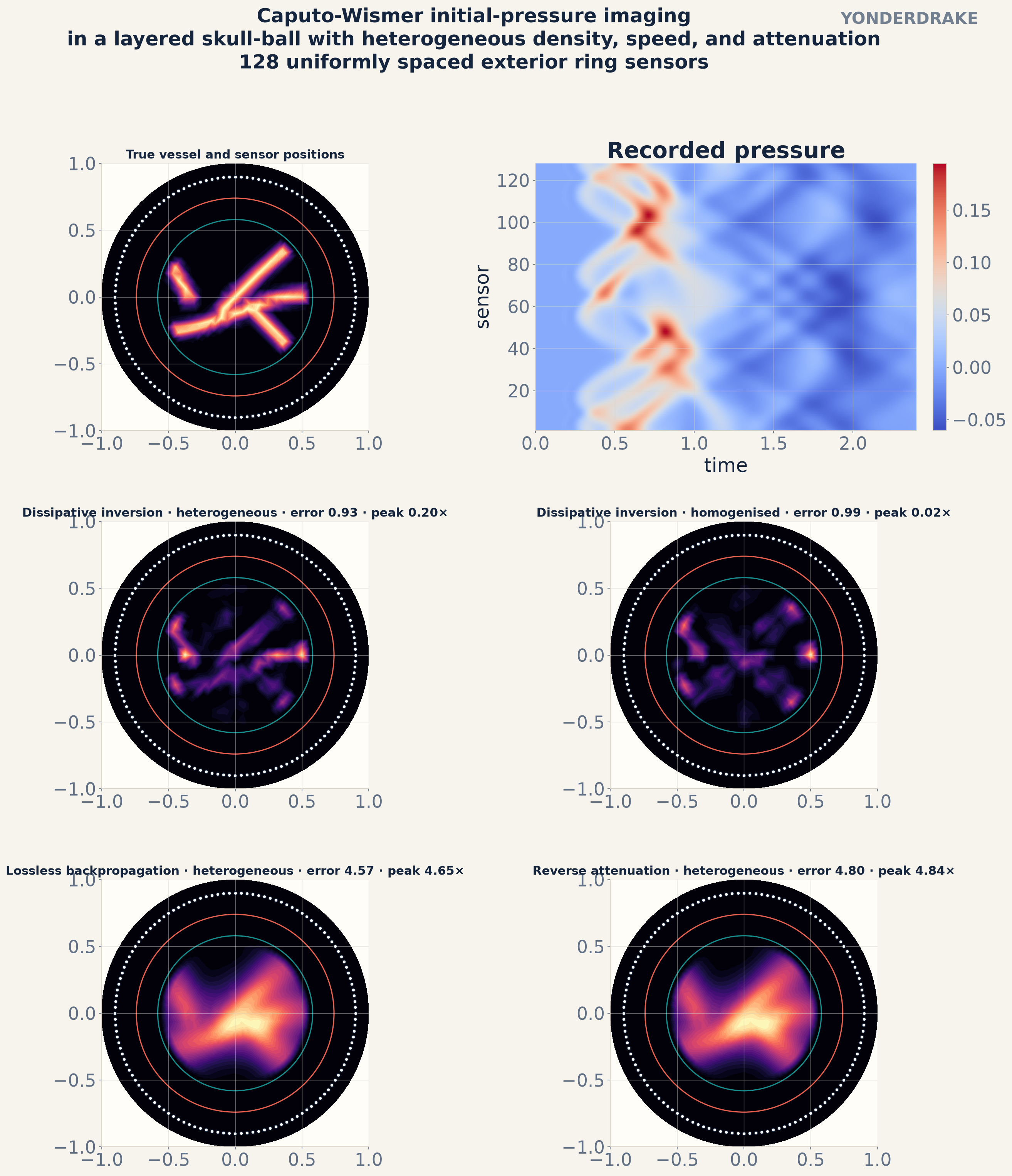
The self-contained layered ball uses the same vessel-source experiment with a circular sensor array. The middle row isolates the effect of using the correct layered material map. The lower row compares lossless and compensated backpropagation through that map. Each reconstruction is scaled inside the tissue region for visibility. The relative error and recovered peak retain the physical amplitude comparison, with lower error being better.

Fractional space

Three Laplacians on a Koch snowflake

visual_fractional_heat_snowflake.py compares classical, spectral-fractional, and Riesz heat flow on the same fractal domain, from the same initial data. The three panels diverge fastest near the boundary, where the two fractional realizations disagree (why).

Surface and plan views of the three operators near the fractal boundary.

A maze seen by three Laplacians

visual_fractional_maze.py places an equal source and sink at opposite ends of a branching maze and solves

\[ \mathcal{A}u=q_{\mathrm{start}}-q_{\mathrm{goal}}. \]

The blue start is the source and the black goal star is the sink. The forcing has zero integral. The classical and spectral operators use reflecting walls, and their potentials have zero mean. The restricted Riesz operator retains its zero-exterior realization. The classical construction is inspired by Connolly, Burns, and Weiss and the FiniteVolumeMethod.jl maze tutorial.

The classical flux \(-\nabla u\) follows the unique connected route from start to goal and vanishes in dead ends. The spectral field follows the topology of the Neumann Laplacian but redistributes the response nonlocally. The restricted Riesz field can couple corridors that are close in Euclidean space but separated by a wall. The plots show \(|\nabla u|\), which reveals where each equilibrium field changes through the maze.

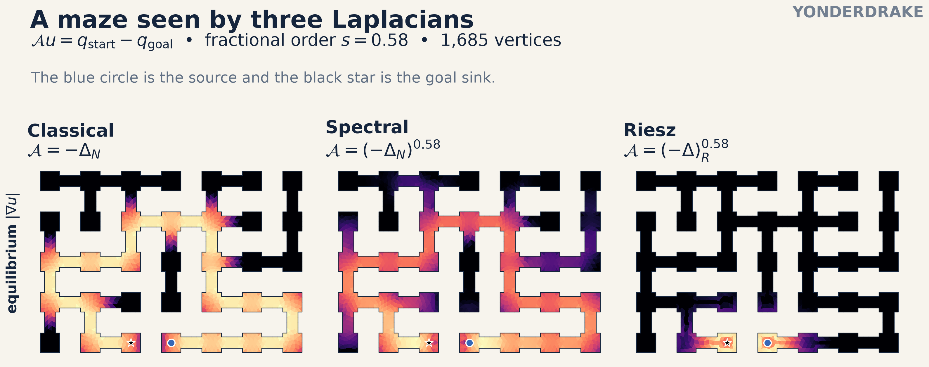
Equilibrium gradient magnitude for the classical, spectral-fractional, and restricted Riesz realizations.

The same comparison can be viewed as a transient problem. Starting from zero, the three fields solve

\[ \partial_t u + \mathcal{A}u=q_{\mathrm{start}}-q_{\mathrm{goal}} \]

and approach equilibrium. Small initial timesteps resolve the advancing front, then progressively larger timesteps follow the slower approach to the established path. Each panel keeps its equilibrium gradient scale throughout the animation.

Transient classical, spectral fractional, and restricted Riesz responses to the same start source and goal sink.

A fractional race through a periodic gyroid

visual_periodic_fractional_gyroid.py races two copies of the same multiscale implicit surface through a fully periodic 3D box. The lower spatial order retains fine modes while the near-local order rapidly exposes the broad gyroid scaffold. Both fields use the 3D PeriodicFractionalLaplacian.

The zero isosurfaces rotate together while their small-scale structure dissipates at different rates. The black slice contours track the same level set through each periodic cell.

Fractional Schrödinger on an aperiodic monotile

visual_fractional_schrodinger_monotile.py solves four Schrödinger models on a hat monotile patch: classical, space fractional, time fractional, and fully fractional. The spatial operator is the Dirichlet spectral fractional Laplacian, so the panels compare realizations on a bounded domain. Because complex PETSc builds are rejected (Supported platforms and dependencies), this is solved as a coupled real system. This and the head demos use CG2.

The coupled real fields evolve across the nonperiodic hat-monotile patch.