Mathematics and Implementation
The supported time derivatives and their memory representations are described together below. Power-law memory uses either stored history or diffusive modes. Single-exponential memory is a bounded-kernel fading-memory operator with one exact state and no quadrature spectrum. It shares the time-memory interface.
How those modes are advanced alongside the field is a separate choice, covered in How the memory is advanced.
Caputo and Riemann-Liouville derivatives
Both time derivatives are symbolic markers. They record which derivative you want. The representation and formulation decide how it is computed. Orders are immutable and satisfy \(0<\alpha<1\).
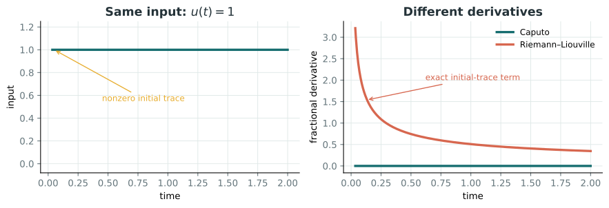
For the same constant input, Caputo annihilates the initial value while the Riemann-Liouville derivative retains its singular initial-trace term.
Caputo
For a sufficiently regular \(u\),
CaputoDerivative(u, alpha) marks this. The Caputo derivative of a constant
is zero, so classical initial data need no special treatment.
Riemann-Liouville
The supported left derivative with lower limit \(t_0\) is
and for a \(u\) with a classical trace at \(t_0\) it splits as
RiemannLiouvilleDerivative(u, alpha) approximates the Caputo part with the
chosen representation and adds the initial-trace term exactly. A nonzero
constant retains this trace contribution.
Construction snapshots \(t_0\) and \(u(t_0)\). reset(u0, t0=...) replaces both.
Evaluation at \(t_0\), arbitrary prehistory, and fractional-integral initial
data are not currently supported. The equivalence used here follows
Yuan, Gao, Xiu, and Shi (2020).
Markers must wrap the stepped field
Marker replacement happens before form compilation and differentiation, so the
marker has to sit directly on u. Fixed spatial UFL operators may surround
it:
Du = CaputoDerivative(u, alpha)
F_damping = b * inner(grad(Du), grad(v)) * dx
This is the weak form of \(-b\Delta D_C^\alpha u\). Wrapping a transformed
expression instead of u is currently unsupported.
The justification is commutation. Let \(L\) be a linear, time-independent spatial operator on a fixed domain. If \(u\) is regular enough for \(L\) to pass through the defining integral, then
and for the Riemann-Liouville marker the classical trace must additionally lie in the domain of \(L\). Time-dependent or nonlinear spatial operators, moving domains, and incompatible boundary realizations break this and are unsupported.
Multi-term damping
With fixed indicator functions \(\chi_m(x)\) over a material partition, the recurrence path supports several orders in one residual:
Each order owns its own diffusive representation. All terms share the field and the time increment. The head demos in the Gallery use this form.
Diffusive representations of time memory
A Caputo derivative depends on the whole history of \(u\). Most diffusive methods replace that history by a fixed number of first-order memory modes,
with positive rates \(\lambda_j\) and weights \(w_j\) obtained by quadrature of
Storage is \(O(m)\) per fractional term. These positive-rate methods differ in
how that improper integral is discretized. SineDiffusive uses the separate
undamped construction described below.
Representation |
Quadrature |
Status |
Source |
|---|---|---|---|
|
Gauss-Jacobi after a Cayley map of selectable exponent |
Default |
Generalizes Diethelm (2008) and Birk and Song (2010) |
|
Gauss-Jacobi after a two-parameter endpoint map |
Expert |
|
|
Dyadic Gaussian construction over a requested interval |
Supported alternative |
|
|
Published Gauss-Laguerre rule, or truncated trapezoidal/Simpson/Gauss-Legendre rules |
Comparison only |
|
|
Original Gauss-Laguerre rule |
Comparison only |
|
|
Generalized Gauss-Laguerre quadrature of sine modes |
Comparison only |
The Gauss-Jacobi family
Cayley maps the semi-infinite rate axis onto the Gauss-Jacobi reference
interval. Writing \(r=(1-x)/(1+x)\) and taking rates \(\lambda=r^{p}\), the
integral above becomes
a Jacobi weight against a smooth remainder, which is what makes the rule converge geometrically rather than at the root-exponential rate the semi-infinite constructions achieve. Both exponents exceed \(-1\) for every \(p>0\) and every \(\alpha\in(0,1)\).
That exponent sets how many decades of relaxation rate a given mode count
spans, so a larger \(p\) reaches further but resolves each decade less finely.
The best \(p\) follows the width of the rate window the problem needs and
barely moves with \(\alpha\). Give Cayley a t_final and a min_step and it
sizes the exponent from that declared span. Alternatively, give it power
directly to set the exponent yourself (except for exactly \(1\) because that
places the Jacobi exponents on the degenerate \(\alpha+\beta=-1\) recurrence).
Two of these exponents are published as methods and are available under their
own names: Diethelm2008(n) is Cayley(n, power=2) and BirkSong(n) is
Cayley(n, power=4).
Nothing forces the two ends of the map to share an exponent. Taking
\(\lambda(x)=(1-x)^{\sigma}/(1+x)^{\rho}\) gives Jacobi exponents
\(\sigma\alpha-1\) and \(\rho(1-\alpha)-1\), which exceed \(-1\) for every positive
\(\sigma\) and \(\rho\), so the whole two-parameter family is admissible.
Yonderdrake implements it as Jacobi(n, sigma=..., rho=...), with
\(\sigma=\rho=p\) recovering Cayley(n, power=p). Larger \(\sigma\) extends the
long-memory end and larger \(\rho\) the short-memory end, so the two can be
tuned against each other.
Jacobi is an expert option. Its parameters are supplied manually and should
be chosen by measuring kernel error across the time interval and orders the
problem needs, because the diagonal calibration that Cayley uses does not obviously
carry over. At each order the pair is rejected when
\(\sigma\alpha+\rho(1-\alpha)=1\), where the recurrence degenerates.
Mode counts above the recommended ranges remain available for convergence
experiments. Construction emits ModeCountAdvisoryWarning and records
mode_count_recommended=False in the metadata. The larger hard ceilings in
API and supported scope are resource guards. The Gauss-Jacobi construction computes
selected eigenvectors in bounded-size chunks, so its temporary memory grows
linearly with the mode count even though its work remains quadratic.
For Diethelm2022, quadrature="gauss-laguerre" is the quadrature published
with the 2022 representation. Each Laguerre node produces one mode from each
half of the real-line integral, so num_modes must be even and is twice the
Laguerre node count. This canonical construction has no truncation radius or
rate scaling. It rejects the controls that belong only to truncated rules.
Large orders and mode counts can also exceed the range of positive float64
rates or weights, in which case construction raises an error naming the order
and total mode count.
The "trapezoidal", "simpson", and "gauss-legendre" choices instead
truncate the log-rate integral. These variants follow the 2024 analyses by
Chaudhary and Diethelm and
Chaudhary and Diethelm.
Their truncation and envelope controls do not apply to Gauss-Laguerre.
Sum of exponentials on a declared interval
SumOfExponentials derives its mode count from the requested accuracy and
time range:
representation = SumOfExponentials(
    target_error=1e-6,
    min_step=0.01,
    t_final=2.0,
)
The Jiang construction approximates \(t^{-1-\alpha}\) by positive
exponentials on [min_step, t_final]. Yonderdrake converts the same Gaussian
nodes to the Caputo memory weights. The newest interval retains the exact L1
coefficient and the modes carry the older history. This preserves the kernel
singularity without storing the full solution history.
The achieved num_modes is reported by spectrum(alpha).metadata and can
differ between fractional orders. A step below min_step or an advance past
t_final raises an error.
Sine diffusive oscillators
SineDiffusive represents the Caputo derivative as
Each quadrature node stores the pair \((\omega,\dot\omega)\). The Oscillator
formulation advances that pair by an exact rotation and integrates a linear
change in \(u\) exactly over each step.
Generalized Gauss-Laguerre nodes and effective weights are evaluated in log scale beyond the recommended range, where the weighted SciPy values begin to underflow. This keeps finite positive spectra available for high-mode comparison experiments.
stepper = FractionalTimeStepper(
    F,
    SineDiffusive(128),
    t,
    dt,
    u,
    formulation=Oscillator(),
)
The formulation is selected automatically when formulation is omitted.
Ordinary SDR converges only as \(O(m^{\alpha-1})\). Fixed-problem comparisons
against FullHistory also show persistent, oscillatory long-time error because
the modes do not contract. It is included for reproducing and comparing
literature methods. The general time steppers support it. The Caputo-Wismer
application layer supports the positive-rate representations.
Refining a representation
For the fixed-count positive-rate methods, the mode count and rate_scale are
quadrature
parameters of the memory integral. They are independent of the time grid.
Halving dt does not improve a badly resolved spectrum, and adding modes does
not fix a coarse timestep. For SumOfExponentials, lower target_error to
derive a finer spectrum, then lower dt and rebuild the representation with
the new min_step. Refine one control at a time, as in
Refinement workflow.
For SineDiffusive, increase the mode count at fixed dt first. Its slow
quadrature convergence and undamped long-time error should both be measured
against FullHistory on the intended time interval.
Equal mode counts across representations do not imply equal accuracy. Comparisons are only meaningful against a shared analytic or high-accuracy reference. See Time-memory representations for the comparison.
Direct convolution methods
The diffusive representations replace the power-law kernel with a fixed set of memory modes. Yonderdrake also provides three uniform-grid methods that act on the convolution itself. They are useful when a published discretization is part of the model, when second-order time accuracy is important, or when a long run makes direct history too expensive.
Lubich convolution quadrature
LubichCQ generates convolution weights from a backward
difference symbol. For the Caputo derivative, it applies the weights to
\(u-u(0)\):
The available symbols are
BDF2 is the default. num_corrections adds Lubich starting weights that are
exact for the first powers \(t^{\alpha},t^{2\alpha},\ldots\). The default is one
correction for BDF1 and two for BDF2.
It uses \(O(n)\) distributed-field storage and \(O(n)\) work at step \(n\), giving \(O(N^2)\) total history work. It requires a uniform timestep. BDF2 gives second-order convergence for sufficiently regular data. Initial singularities can reduce the observed order, which is why the starting corrections are part of the default.
Alikhanov L2-1-sigma
AlikhanovL21Sigma uses Alikhanov’s quadratic L2-1\(\sigma\) approximation with
The complete residual is evaluated at \(t_{n+\sigma}\). Yonderdrake therefore replaces an ordinary occurrence of the solution by \(\sigma u_{n+1}+(1-\sigma)u_n\) and replaces the symbolic time by \(t_n+\sigma h\). The fractional marker and every other term consequently use the same offset equation.
The method is second order on smooth solutions and usually retains better accuracy than uncorrected high-order formulas near a weak initial singularity. It requires a uniform timestep, Caputo markers with one shared \(\alpha\), and stores the full increment history. Its storage and total history work are \(O(N)\) fields and \(O(N^2)\) respectively.
Fast oblivious convolution quadrature
FastObliviousCQ accelerates BDF1 convolution quadrature.
Recent increments are applied exactly. Older increments are grouped into
dyadic blocks and integrated on conjugate Talbot contours. Complex contour
states are represented internally by coupled real arrays, so the public
Firedrake problem still uses real scalar fields.
For \(N\) accepted steps, the history has \(O(\log N)\) work per step and \(O(\log N)\) distributed-field storage, giving \(O(N\log N)\) total history work. The constants include the contour nodes at every active level, so direct history can remain smaller and faster for short runs. The time discretization is BDF1 and is therefore first order.
The principal controls are:
Control |
Meaning |
|---|---|
|
Selects the default number of contour nodes |
|
Explicit contour quadrature size per dyadic level |
|
Number of recent increments kept exact |
|
Dyadic depth, supporting at most \(2^{\mathtt{num\_levels}}-1\) steps |
|
Currently the published |
The method requires a uniform timestep. Increase nodes_per_level to check
contour convergence independently of timestep convergence. Increase
num_levels before a run if its configured maximum step count is too small.
Choosing a time-memory method
BirkSong remains the general default because it has fixed storage and accepts
variable timesteps. Use FullHistory as a direct variable-step reference.
Use BDF2 LubichCQ for classical uniform-grid convolution
quadrature, and AlikhanovL21Sigma when the offset second-order PDE formula is
appropriate. Use fast-oblivious CQ for long uniform-grid histories where its
logarithmic scaling outweighs its contour-state constants.
Exponential (fading) memory
ExponentialMemory(u, decay_rate) represents
It is nonlocal in \(u\), but a single internal state carries its complete history:
This is one mode of the diffusive representation used on its own. Its bounded kernel decays on one timescale and does not follow a power law. Yonderdrake exposes it as fading memory.
Exactness
For a step \(h\) and Yonderdrake’s linear time interpolant, the mode recurrence is exact:
The operator therefore costs one stored field per marker and contributes no quadrature error of its own. Unlike the fractional representations, there is no mode count to refine.
Caputo-Fabrizio
CaputoFabrizioOperator(u, alpha, normalization=1.0) supplies the
parameterization proposed by
Caputo and Fabrizio (2015), which is
exactly a rescaled exponential memory:
for \(0<\alpha<1\) and positive normalization \(B(\alpha)\). Yonderdrake builds it directly from the marker above.
Its rational transfer function is a one-pole high-pass filter. See
Ortigueira and Machado (2018).
Power-law kernels use the representations described under
Caputo and Riemann-Liouville derivatives and are
selected with CaputoDerivative. Refining the exponential model preserves its
one-timescale kernel.
Stepping
Use TimeMemoryStepper for exponential-memory markers:
from yonderdrake import ExponentialMemory, TimeMemoryStepper

F = (inner(ExponentialMemory(u, 1.7), v) - inner(source, v)) * dx
stepper = TimeMemoryStepper(F, t, dt, u)
The default recurrence can mix exponential and fractional markers.
representation supplies the modes for the fractional terms. AuxiliaryODE
supports exactly one exponential marker.
Passing an exponential marker to FractionalTimeStepper raises ValueError,
and FullHistory cannot be combined with it. A worked example is in
Exponential memory and Caputo-Fabrizio.
Warning
The operator is zero at \(t=t_0\), so construction emits an
ExponentialMemoryCompatibilityWarning. An equation using it as the leading
time operator requires the remaining residual and the initial data to satisfy
the corresponding compatibility condition. Check that before setting
warn_initial_compatibility=False. That restriction on admissible initial
data, and the wider question of whether to model with nonsingular kernels at
all, are discussed in
Diethelm, Garrappa, Giusti, and Stynes (2020).