Accuracy and performance

These comparisons show how the numerical controls affect accuracy, setup cost, repeated work, and storage. Absolute timings depend on the machine, mesh, solver configuration, and MPI layout. The trends are the useful part.

The benchmark sources and recorded CSV data are available for reproducing the figures or making a comparison on different hardware.

Question	Measurement	Practical consequence
How many memory modes are enough?	Error against analytic fractional derivatives with no timestep or PDE error	Increase \(L\) until the quantity of interest stops changing, then refine the timestep
What controls time-stepping cost?	Setup and steady cost while varying \(h\), \(\Delta t\), and \(L\) separately	Mesh size controls each solve, \(L\) controls memory work and storage, and \(\Delta t\) controls how many solves are needed
How accurate are the spatial numerical controls?	Error against an analytic spectral power or an over-resolved Riesz action	Tighten the operator control until its error is below the mesh error
What is paid once and what is paid repeatedly?	First application and cached application timings	Setup matters for short jobs, while repeated cost matters for long integrations and inverse problems
Which Riesz backend fits the problem?	Construction, application, storage, and agreement with dense assembly	Matrix-free avoids storage, H-matrices trade compression error and setup for faster reuse, and dense assembly is a small-problem reference

Time-memory representations

The first comparison applies every supported and comparison-only time-memory representation to the same two analytic functions over six decades of time. The fixed-count methods use 40 or 41 modes to respect the even-count Gauss-Laguerre and odd-count Simpson rules. SumOfExponentials derives its mode count from a \(10^{-4}\) kernel target on the declared interval. Its newest interval uses the same linear-interpolant correction as the time stepper, with min_step=1e-5. The fixed-count modes are evaluated analytically. The curves therefore measure the standalone derivative approximation without a PDE mesh or linear solver.

The fixed-count methods use 40 or 41 modes. The sum of exponentials uses the mode count selected by its requested tolerance and interval.

Spectrum construction is a small setup cost. Preparing the recurrence coefficients is cheaper still. The sum of exponentials includes the cost of deriving its tolerance-controlled spectrum.

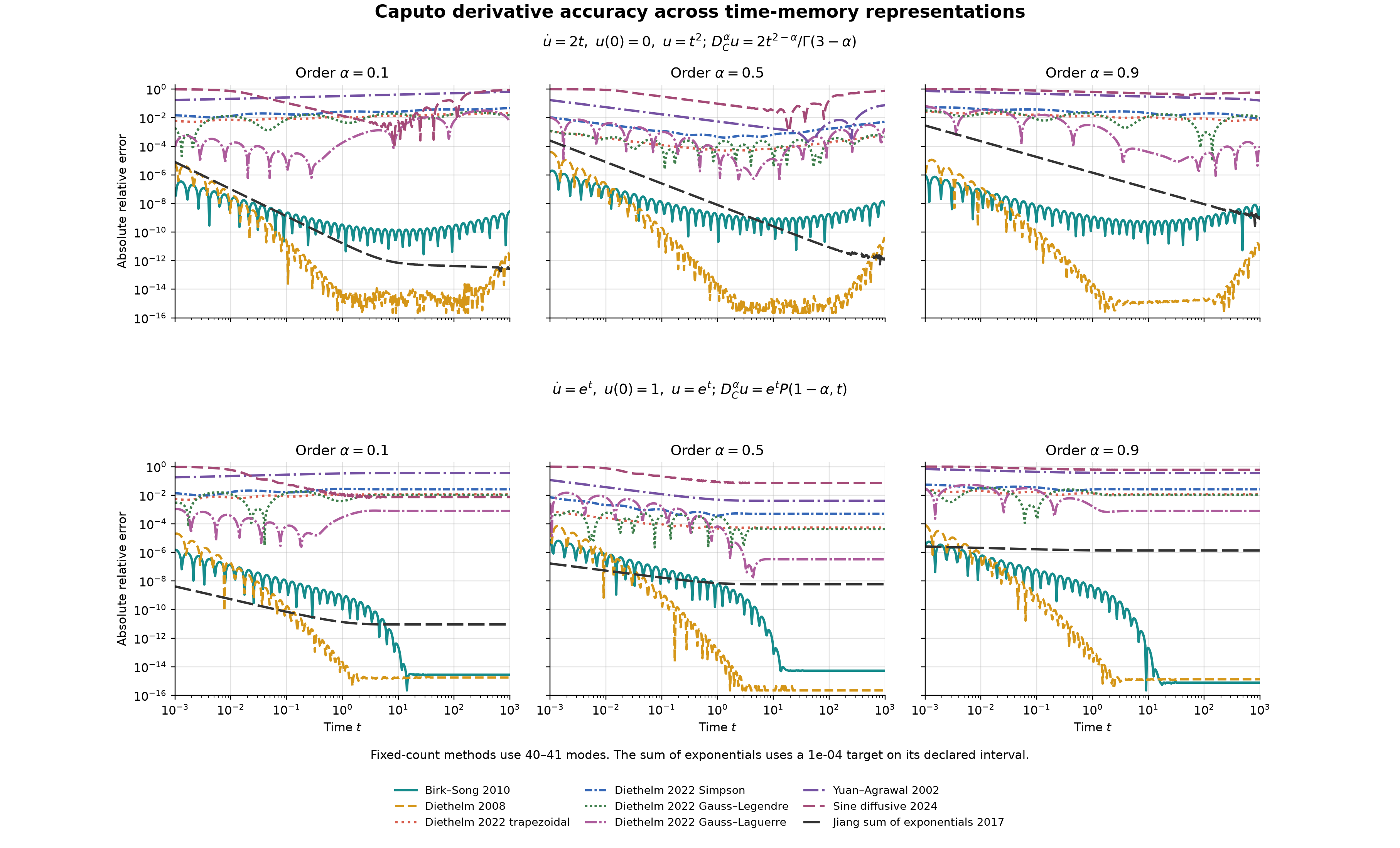
BirkSong is the default. Diethelm2008 and SumOfExponentials are supported alternatives. Diethelm2022, YuanAgrawal, and SineDiffusive are literature-comparison options. The large differences in their curves come from the placement and scaling of the modes over the problem’s time range. Mode count alone does not determine accuracy.

SineDiffusive uses exact undamped rotations. The other rows use a decaying first-order update. Its slow mode refinement and persistent long-time error are visible in the results.

Accuracy at matched computational cost

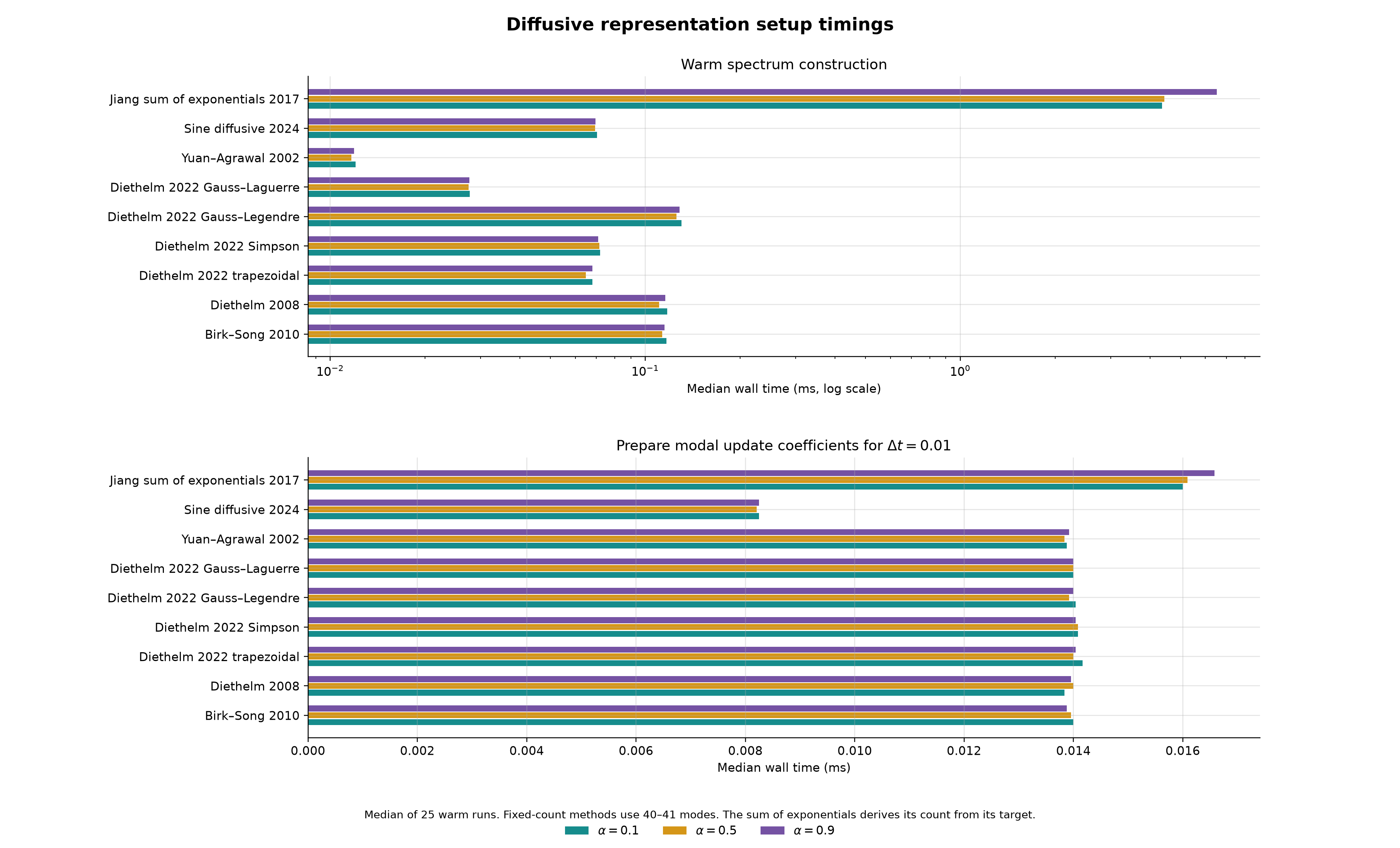
Equal mode counts are close to equal cost for the positive-rate methods because they use the same static-memory recurrence. The sine representation stores and advances two states per frequency. The cost-matched comparison therefore calibrates each fixed-count method against the same measured workload.

The reference budget is the mean time for 41-mode Birk-Song and Diethelm. A workload includes spectrum setup and 512 static-memory updates over 256 scalar field values at each of the three fractional orders. Each fixed-count method uses the valid total mode count with the nearest median runtime. For SumOfExponentials, the requested tolerance is selected from a logarithmic sequence and its derived spectrum is timed in the same workload. The legend reports every selected count and measured cost ratio.

This comparison uses \(0.1\leq t\leq10\). Over that representative interval the derived sum-of-exponentials spectrum fits the same moderate work budget, while Birk-Song and Diethelm remain above floating-point saturation for enough of the range to compare errors above the machine-precision plateau.

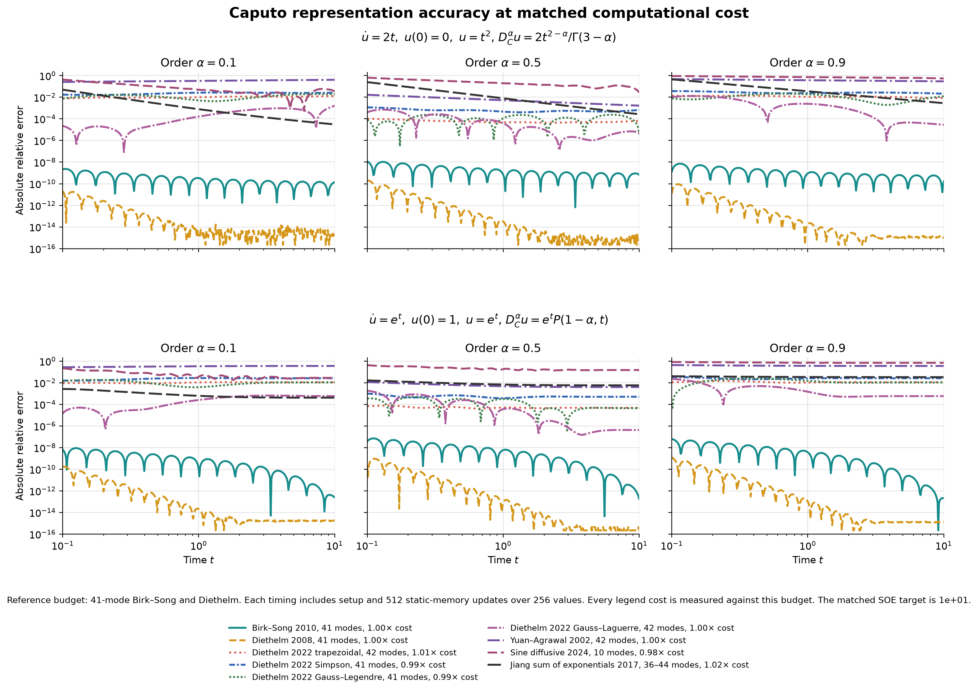
Representation error for two analytic Caputo derivatives at the same measured memory-work budget.

The fixed-count error curves use exact auxiliary-mode evolution. The sum of exponentials includes its required newest-interval correction. The comparison isolates the accuracy bought by the representation-controlled work without a mesh, solver, or PDE error. A full PDE also pays for its common linear solve, so differences in total application runtime will be smaller.

Accuracy across time-memory families

The representation comparison above isolates spectrum error. The end-to-end comparison below measures actual Firedrake solves for the manufactured solutions \(u(t)=t^2\) and \(u(t)=t^\alpha\), including construction, history updates, and linear solves. The reference budget is the mean wall time of fixed 100-mode Birk-Song and Diethelm 2008 runs. Each run advances 500 timesteps with \(\Delta t=0.001\) over \(0 \leq t \leq 0.5\). Every other family uses the same time grid and is tuned only within 0.5 to 2 times that measured budget. The candidate with the smaller worst error is then retained. The two reference methods themselves remain fixed at 100 modes.

The benchmark varies mode count and scale for fixed spectra, tolerance for the sum of exponentials, order and starting corrections for Lubich CQ, and contour size and direct window for fast-oblivious CQ. The timestep and physical interval remain fixed. These timings cover the complete time-memory method. The earlier figure covers quadrature alone.

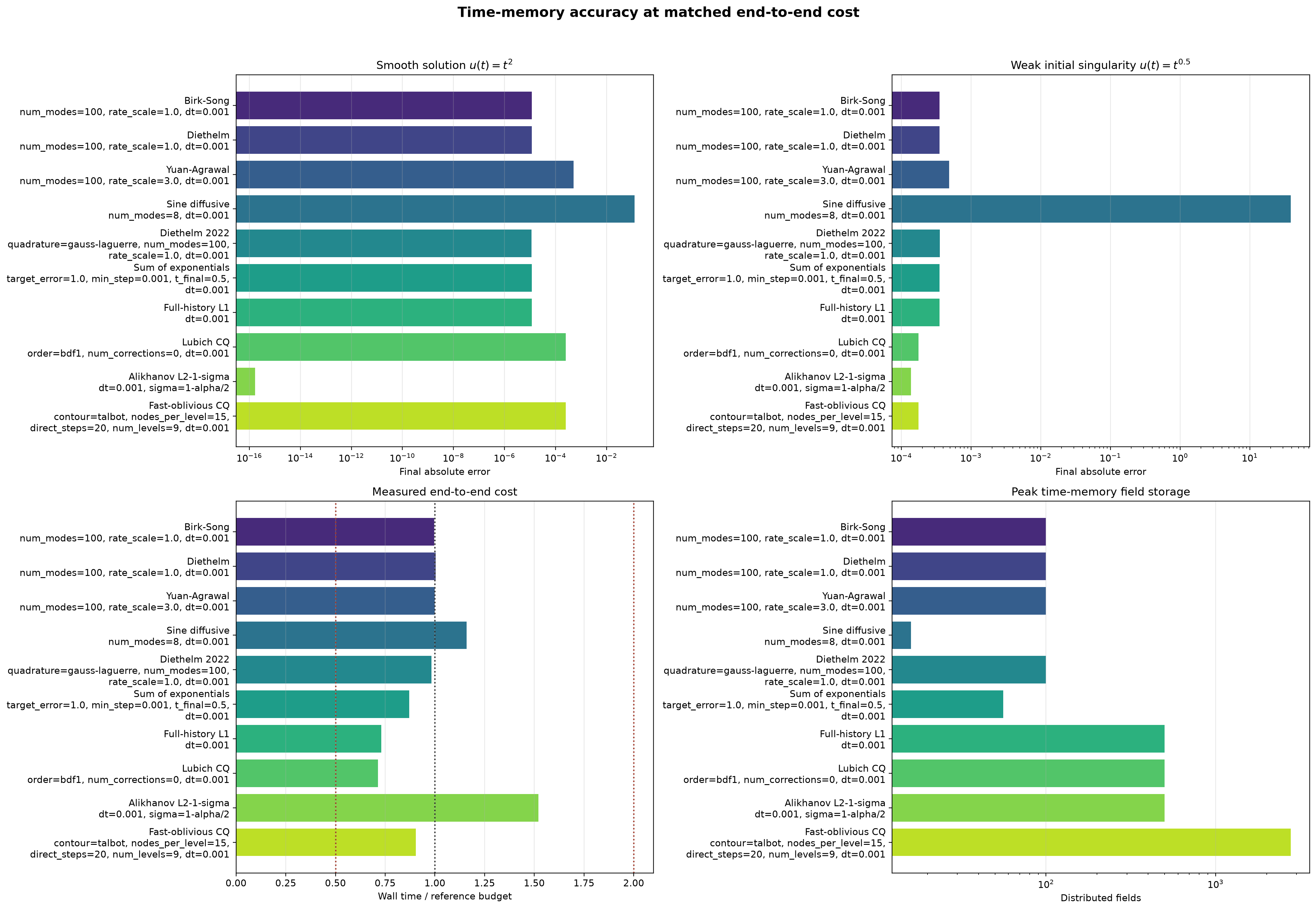
Accuracy, measured end-to-end cost, and peak distributed-field storage for the selected method configurations. The CSV records every selected parameter, runtime ratio, error, and asymptotic work and storage class.

Convergence with mode count

The Diethelm 2008 refinement study holds the time treatment fixed and increases only the number of Gauss-Jacobi nodes. More nodes extend the interval over which the representation remains accurate and lower the error until floating-point precision becomes visible.

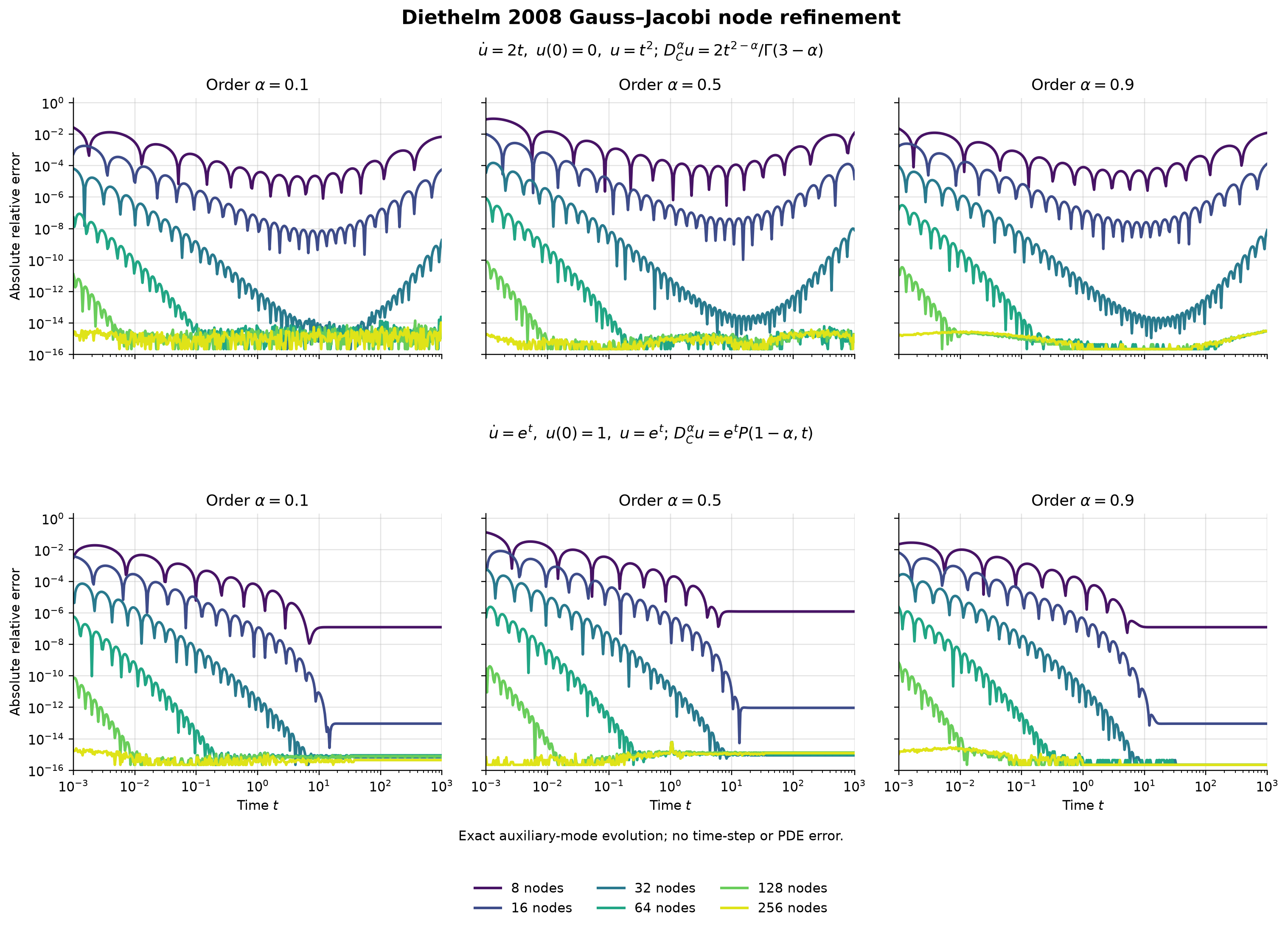
Diethelm 2008 node refinement for polynomial and exponential inputs at three fractional orders. Each curve contains representation error only.

For an application, first increase \(L\) at fixed \(\Delta t\). Once that result is stable, reduce \(\Delta t\) to measure the separate time-discretization error. The refining workflow gives the corresponding sequence for every operator family.

Tolerance-driven exponential sums

SumOfExponentials appears in the shared comparisons with a mode count derived from its requested interval and tolerance. The study below isolates that control by tightening the absolute kernel target on a fixed interval and recording the verified error, derived storage, and construction cost.

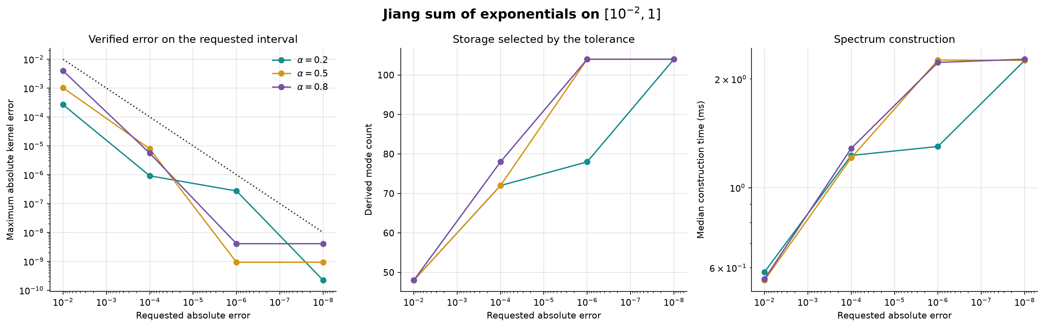
Tighter kernel tolerances derive more modes. The verified error remains below the requested target for each tested fractional order.

Fractional time stepping

The application study uses two different PDEs. The thermal problem is a moving heat source on a torus. The Caputo-Wismer problem is a wave travelling through a layered skull geometry with an absorbing exterior boundary. Each study changes the mesh size \(h\), timestep \(\Delta t\), or number of diffusive nodes \(L\) while holding the other two fixed.

Construction and the first step grow mainly with the physical problem size. Birk-Song and Diethelm have similar setup costs in these applications.

Mesh refinement raises the cost of each step. Increasing $L$ adds memory work, while changing $\Delta t$ has no systematic effect on the cost of one step.

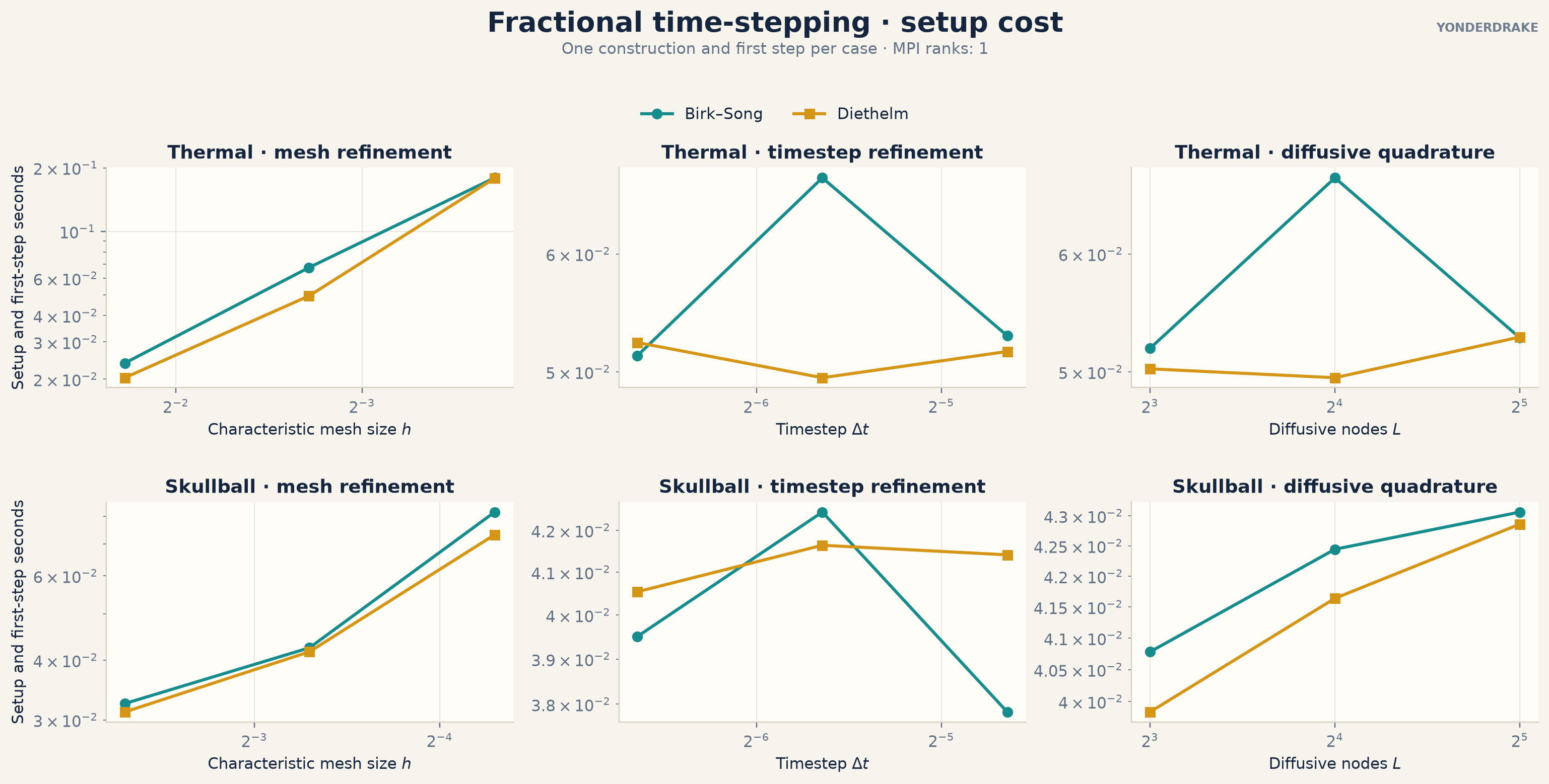
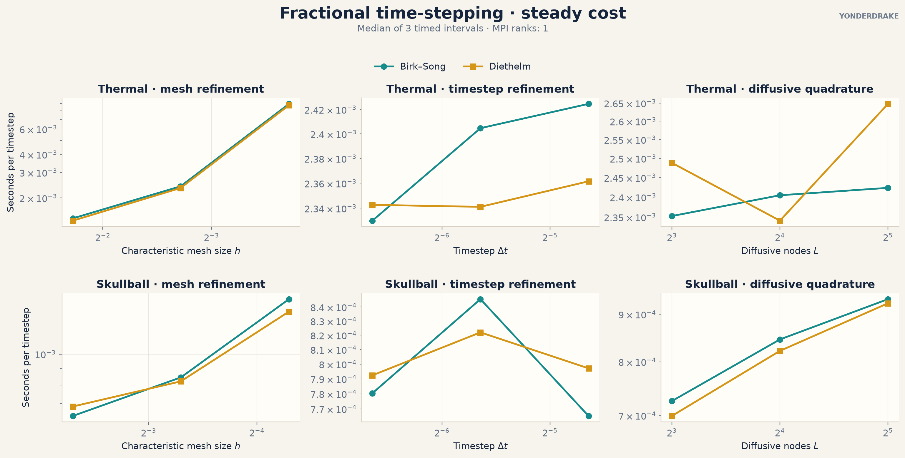
The timestep still has a direct effect on total runtime. Halving \(\Delta t\) approximately doubles the number of steps needed to cover the same physical duration, even when the cost of each step is unchanged.

For a field with \(N\) degrees of freedom and one fractional term, static memory stores \(LN\) mode values. Doubling \(L\) therefore doubles that memory state. Multiple fractional terms contribute their own mode fields. See Performance and MPI for the storage requirements of the other formulations and spatial operators.

Spatial fractional operators

The spatial results separate three effects that should be refined independently:

1. the finite-element mesh

2. the internal approximation used to apply the nonlocal operator

3. the algebraic solver tolerance.

The figures below vary the first two. Solver tolerances are kept below the measured numerical error.

Accuracy of the internal controls

For the spectral operator, the sinc truncation target controls the number of shifted elliptic solves. Tightening it reduces the error against a known fractional eigenvalue power. For the Riesz operator, increasing the target quadrature degree reduces the error against an over-resolved Galerkin action.

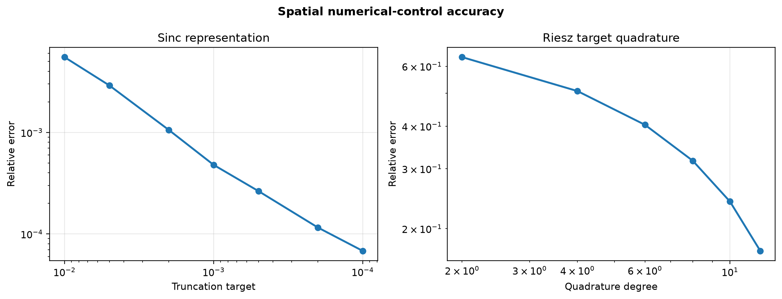
Numerical-control error on fixed meshes. These curves do not include a mesh refinement study.

The seven-point spectral sequence behaves like an accuracy request in this test, with the observed error falling as the requested target is tightened. Riesz target quadrature is shown at six degrees. It converges more gradually and becomes increasingly expensive. In both cases, further refinement is useful only while this error is large enough to affect the final solution.

The periodic Fourier operator has no quadrature control. Its accuracy is set by the resolution of the uniform periodic grid, and its action uses a distributed FFT. Refining that grid increases both the resolved wavenumber range and the FFT work.

Mesh and operator scaling

The scaling comparison uses the irregular-island geometry and population field from the habitat example. The mesh panel compares repeated spectral and matrix-free Riesz actions at six mesh resolutions. The other panels hold the mesh fixed and use six values of each operator-specific numerical control.

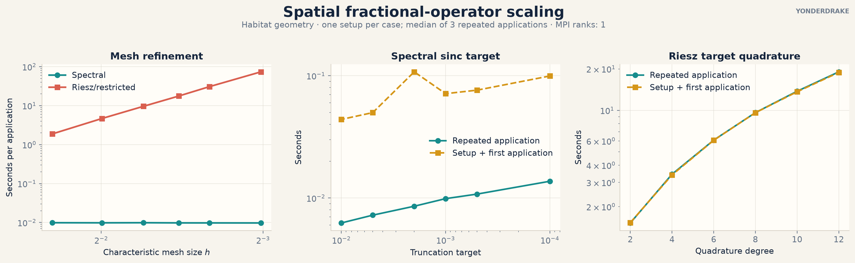
Setup and repeated-application costs for the spectral and matrix-free Riesz operators. The absolute values are serial timings for these particular small problems.

The spectral operator pays for shifted elliptic solvers during setup and then reuses them. A tighter sinc target adds shifts, so setup grows more strongly than a cached application. The Riesz action evaluates a nonlocal integral, so both mesh refinement and higher target quadrature increase repeated work substantially. Across the six plotted meshes, its measured application time rises from 1.9 seconds at 25 degrees of freedom to 73.8 seconds at 121 degrees of freedom. These operators define different boundary and exterior problems, so the timing comparison is useful after the required mathematical realization has been chosen.

Riesz storage and reuse

The three Riesz backends apply the same Galerkin operator with different storage and reuse strategies.

Backend	Construction and storage	Repeated application	Intended use
Matrix-free	No dense nonlocal matrix	Recomputes the integral action	General use and problems where dense storage is unacceptable
H-matrix	Builds dense near blocks and compressed far blocks	Reuses the compressed representation	Repeated applications and larger problems where setup can be amortized
Dense	Builds and stores all weak entries	Very cheap after assembly	Reference calculations on small problems

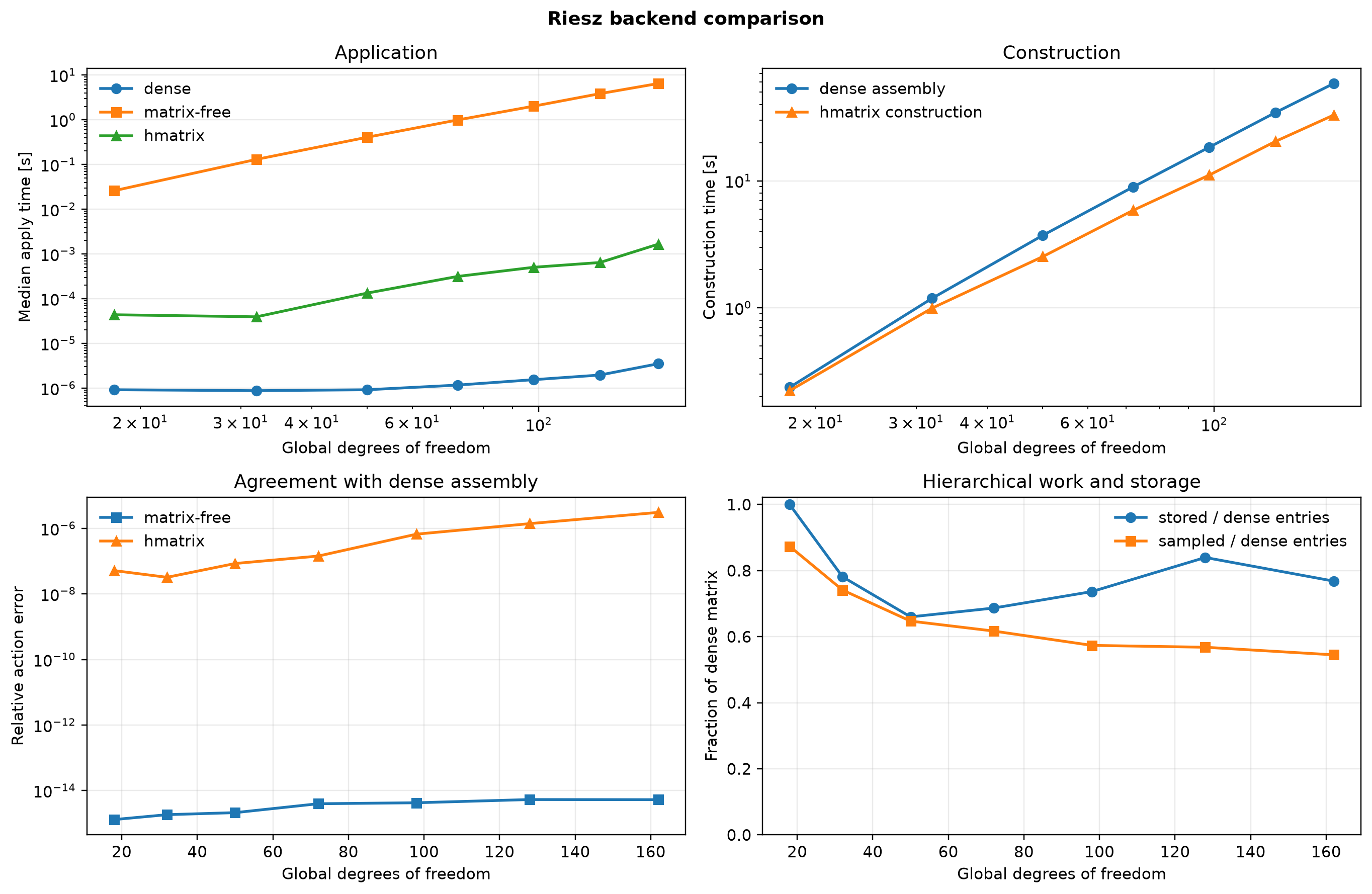
Application time, construction time, agreement with dense assembly, and hierarchical storage at seven separated-patch problem sizes.

Matrix-free agrees with dense assembly to floating-point precision in this study. The H-matrix error follows from compression and remains below \(10^{-5}\) for the tested tolerance. Its construction is cheaper than dense assembly and its repeated action is much cheaper than recomputing the matrix-free integral. The crossover depends on problem geometry, tolerance, mesh size, and how often the operator is applied.