Quickstart

Yonderdrake adds two things to Firedrake: markers you put inside an ordinary UFL residual, and a stepper that knows how to evolve them. Everything else is Firedrake.

A time-fractional ODE to start with

Solve \(D_C^{0.6}u+u=0\), \(u(0)=1\):

import firedrake as fd
from yonderdrake import (
    BirkSong,
    CaputoDerivative,
    Diethelm2008,
    FractionalTimeStepper,
    FullHistory,
)

mesh = fd.UnitIntervalMesh(1)
V = fd.FunctionSpace(mesh, "CG", 1)
u = fd.Function(V).assign(1.0)
v = fd.TestFunction(V)
t = fd.Constant(0.0)
dt = fd.Constant(0.01)

F = (fd.inner(CaputoDerivative(u, 0.6), v) + fd.inner(u, v)) * fd.dx
stepper = FractionalTimeStepper(F, BirkSong(48), t, dt, u)

for _ in range(100):
    stepper.advance()
    t.assign(t + dt)          # the caller updates t after advance()

print(f"u({float(t):.2f}) = {u.dat.data_ro[0]:.6f}")

The final value should be close to 0.41. The exact solution is the Mittag-Leffler value \(E_{0.6}(-1)\). Timestep and representation errors explain the remaining difference.

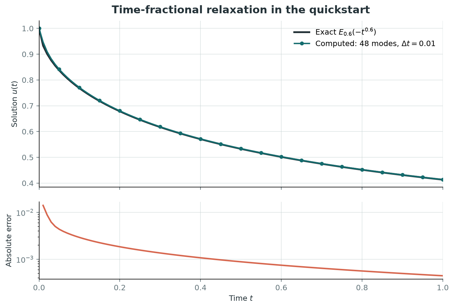
The quickstart computation over \(0\leq t\leq1\), compared with \(E_{0.6}(-t^{0.6})\). The lower panel shows the absolute error on a base-10 logarithmic scale from the same 48-mode Birk-Song calculation with \(\Delta t=0.01\).

Three choices appear here:

Choice	Here	Alternatives
Which derivative	CaputoDerivative	RiemannLiouvilleDerivative
How memory is represented	BirkSong(48)	Diethelm2008, SumOfExponentials, FullHistory
How memory is advanced	default Recurrence	AuxiliaryODE

Swapping a representation means changing one argument:

stepper = FractionalTimeStepper(F, Diethelm2008(48), t, dt, u)
stepper = FractionalTimeStepper(F, FullHistory(), t, dt, u)

Use BirkSong by default or Diethelm2008 as its direct alternative. Use SumOfExponentials when the time interval and an absolute kernel tolerance are known in advance. The remaining diffusive representations are for literature comparisons. See the method map. For single-exponential memory, see Exponential memory and Caputo-Fabrizio.

Adding space

The marker must wrap the stepped field u directly. Fixed spatial operators go around it. For example, a Caputo derivative in time and an ordinary Laplacian in space gives

\[ {}^{\mathrm C}D_t^\alpha u-\kappa\Delta u=f \quad\text{in }\Omega_Y, \qquad u=0\quad\text{on }\partial\Omega_Y. \]

Its weak residual is ordinary UFL with a Yonderdrake time marker:

F = (
    fd.inner(CaputoDerivative(u, alpha), v)
    + kappa * fd.inner(fd.grad(u), fd.grad(v))
    - fd.inner(source, v)
) * fd.dx

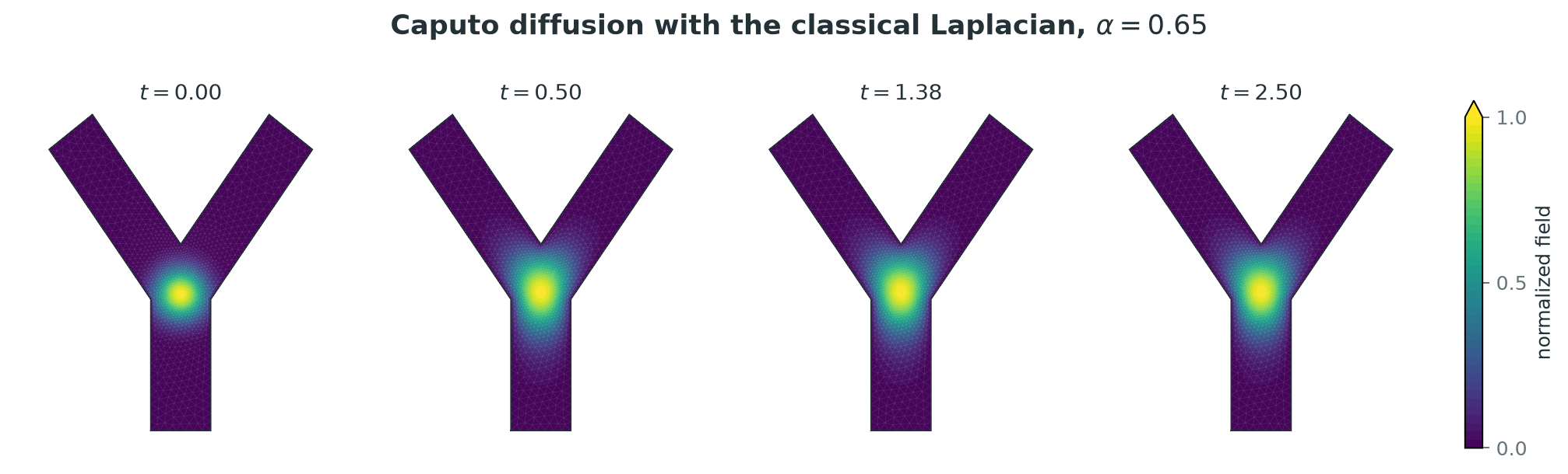
A localized field spreading through a Y-shaped domain under a Caputo time derivative and an ordinary spatial Laplacian. The field lives on a 2D domain, but only the time derivative is fractional in this example.

For a spatially fractional operator, use one of the three spatial operators as an ordinary term in the residual. Replacing the ordinary Laplacian with the homogeneous-Dirichlet spectral fractional Laplacian gives

\[ {}^{\mathrm C}D_t^\alpha u+\kappa(-\Delta_D)^s u=f \quad\text{in }\Omega_Y, \qquad u=0\quad\text{on }\partial\Omega_Y. \]

from yonderdrake import SpectralFractionalLaplacian

bc = fd.DirichletBC(V, 0.0, "on_boundary")
Lu = SpectralFractionalLaplacian(u, 0.4, bcs=bc)
F = (
    fd.inner(CaputoDerivative(u, alpha), v)
    + kappa * fd.inner(Lu, v)
    - fd.inner(source, v)
) * fd.dx

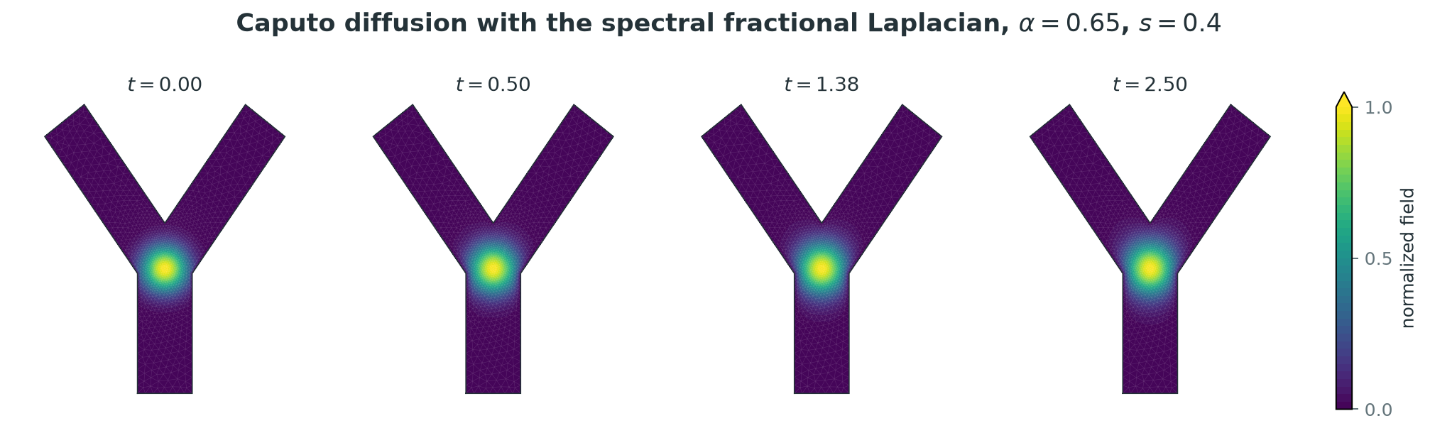
The same initial field under a Caputo time derivative and a spectral fractional Laplacian with \(s=0.4\). Both the time and space operators are nonlocal.

SpectralFractionalLaplacian, RieszFractionalLaplacian, and PeriodicFractionalLaplacian implement three distinct realizations. The model determines which one applies: which one you want.

Controlling numerical error

Fractional problems have more independent error sources than classical ones. Refine one at a time:

Symptom	Control	Note
Memory poorly resolved	mode count, rate_scale	independent of dt
Time discretization	dt	independent of mode count
Spatial discretization	mesh	refine last
Spectral quadrature	sinc_truncation_target	sinc model estimate. Mesh controls FE error
Riesz quadrature	quadrature_degree	separate from compression tolerance
Periodic Fourier	uniform grid size	keep represented modes below Nyquist
Algebraic	PETSc tolerances	keep below the discretization error

Refinement workflow gives a separate refinement sequence for each operator.

Refining the quickstart

Rerun the first example with a finer memory representation and a smaller timestep:

u.assign(1.0)
t.assign(0.0)
dt.assign(0.001)
stepper = FractionalTimeStepper(F, BirkSong(256), t, dt, u)

for _ in range(1000):
    stepper.advance()
    t.assign(t + dt)

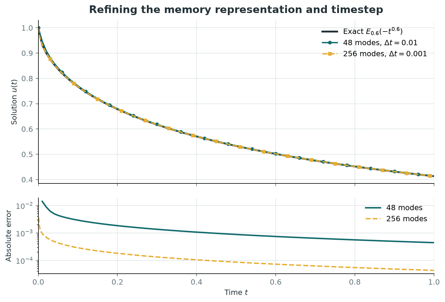
The original calculation uses 48 modes and \(\Delta t=0.01\). The refined calculation uses 256 modes and \(\Delta t=0.001\). Refining both independent controls reduces the error over the full interval.

The refinement costs more work. On our test MacBook Pro with an Apple M3 Pro, the original 100-step loop took about 0.05 seconds. The refined 1,000-step loop took about 1.10 seconds. These are medians of seven warm runs. This is the usual trade-off between accuracy and computational cost.

Common setup problems

Symptom	What to check
The marker is rejected	Wrap the stepped field u directly. Put fixed spatial operators around the marker.
The solution advances but displayed time does not	Update the caller-owned t only after each successful advance().
A periodic operator rejects the mesh	Use a fully periodic, uniform Q1 interval, quadrilateral rectangle, or hexahedral box with at least three cells per direction.
A Riesz operator rejects the space	Use scalar CG1 or CG2 on affine 2D triangles or 3D tetrahedra, and provide complete homogeneous boundary conditions when \(s\geq1/2\).
Sinc construction emits a precision warning	The requested target is below useful float64 resolution. Choose a realistic truncation target and measure mesh error separately.
An imaging demo reaches its iteration cap	Inspect the reported optimizer reason and gradient norm, then raise --inverse-iterations or relax --inverse-tolerance deliberately.

Exact supported combinations and validation rules are collected in API and supported scope.

Notebooks

Two Jupyter notebooks work through complete problems on a graded 2D mesh, building up one step at a time and plotting as they go.

Notebook	What it builds
01-time-fractional-diffusion.ipynb	Graded mesh, a Mittag-Leffler warm-up, the 2D Caputo problem, a manufactured solution, separating mode and timestep error, and graded timesteps
02-spectral-fractional-laplacian.ipynb	The spectral operator on a known eigenfunction, the sinc quadrature knob and its discretization floor, solving \((-\Delta_D)^s u=1\), why grading pays, and coupling back to a Caputo derivative

Run them in an activated Firedrake environment. Beyond Yonderdrake itself, they need only matplotlib and mpmath. They are stored without outputs, so every figure is produced by the run in front of you.

A Jupyter kernel is a single process, so the notebooks run serially however the environment was launched. They show each step of the calculation. For larger problems, use mpiexec -n N python your_script.py, as in demos/. Driving MPI from Jupyter via ipyparallel is currently untested.

Next

• Guides and examples: worked examples, one feature at a time.

• Gallery: larger applications, with animations.

• Mathematics and methods: definitions, methods, and their papers.

• API and supported scope: signatures and exact limitations.